가짜 데이터의 유용함
머신러닝 모델의 성능을 향상시키는 가장 좋은 방법은 더 많은 데이터로 훈련하는 것입니다. 모델이 더 많은 예제로 학습할 수록 이미지 속 차이점이나 중요한 것, 중요하지 않은 것을 잘 찾을 수 있습니다.
그렇게 모델이 새로운 데이터에서도 잘 분류하여 일반화되죠.
데이터를 더 얹는 방법 중 쉬운 방법은 가지고 있는 데이터를 사용하는 것입니다. 분류의 기준을 그대로 지키면서 가지고 있는 데이터를 변형할 수 있다면 그러한 변형을 무시할 수 있는 분류기로 성장시킬 수 있습니다.
예로 자동차의 좌측면과 우측면 사진은 보기엔 다르지만 자동차이지, 트럭이 될 수 없습니다.
그러므로 이런 뒤집힌 사진을 training data에 더해주어(augment) 분류기에게 왼쪽과 오른쪽의 차이점은 무시할 수 있도록 할 것입니다.
그러므로 추가적인 가짜 데이터란, 실제 세계에서 합리적으로 보이지만 분류기가 잡지 못하는 데이터를 의미합니다.
Data Augmentation 사용하기
전형적으로, 많은 종류의 변형들은 데이터셋에 augmenation하기 위해 사용됩니다.
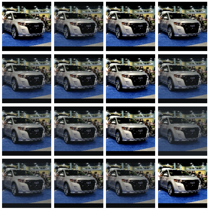
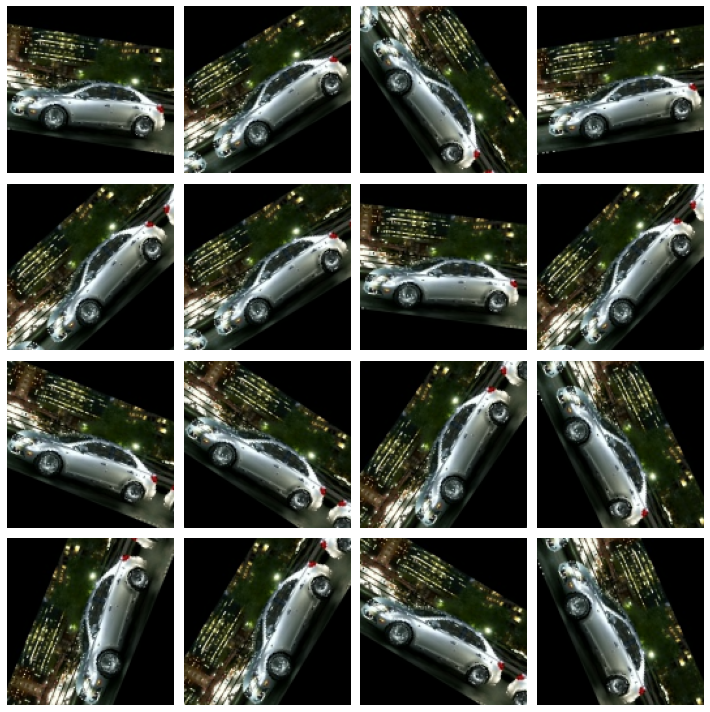
여기에는 이미지를 회전시키거나, 색깔과 대비를 적용하거나, 이미지를 뒤틀거나 등등이 포함됩니다. 보통 이들이 서로 섞여 있죠. 오른쪽 사진은 하나의 이미지가 변형된 예시입니다.
Data augmentation은 보통 온라인에서 합니다. 이는 이미지들이 훈련을 위해 네트워크에 공급된다는 의미입니다. 훈련은 data의 작은 집단(mini-batch)에서 일어난다는 점을 짚고 넘어갑시다.
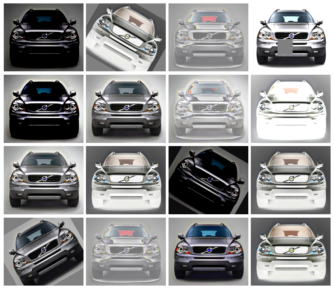
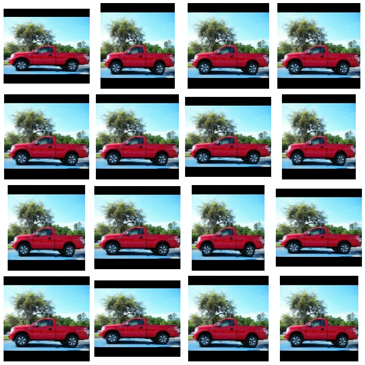
사진은 data augmentation을 할 때 16개의 이미지의 집단의 모습입니다.
매번 하나의 이미지는 훈련하는 동안에 새로운 무작위의 변형을 거쳐갑니다.
이러한 방식으로, 모델은 항상 이전보다 다른 모습을 접하게 됩니다. 이러한 추가한 변형은 training data에 있으며, model이 새로운 데이터에서도 잘 되도록 해줍니다.
모든 변형이 주어진 문제에 유용하지는 않다는 점 또한 중요합니다.
대부분 어떤 변형을 사용하든 집단을 서로 섞지 않아야 합니다.
예로 숫자인식에 대해 훈련 중이라면 9와 6은 이미지를 회전하면 서로 섞일 수 있습니다. 그러니 좋은 augmentation 기법을 찾는 최적의 방법은 해보면서 보는 것밖에 없습니다.
Example - Training with Data Augmentation
케라스에서 augmentation을 두 가지 방식으로 제공합니다.
- ImageDataGenerator 함수로 data pipeline에 추가하기
- 케라스의 preprocessing layer를 사용함으로서 모델 정의에 추가하기
우리가 시도해볼 방법은 두 번째 방법입니다. 가장 좋은 장점은 이미지 변형을 CPU가 아닌 GPU로 하기에 훈련 속도가 증가한다는 점입니다.
이제 첫 수업 때 썼던 분류기를 data augmenation을 써서 향샹시켜봅시다.
1. data pipeline 셋팅
# Imports
import os, warnings
import matplotlib.pyplot as plt
from matplotlib import gridspec

import numpy as np
import tensorflow as tf
from tensorflow.keras.preprocessing import image_dataset_from_directory

# Reproducability
def set_seed(seed=31415):
    np.random.seed(seed)
    tf.random.set_seed(seed)
    os.environ['PYTHONHASHSEED'] = str(seed)
    os.environ['TF_DETERMINISTIC_OPS'] = '1'
set_seed()

# Set Matplotlib defaults
plt.rc('figure', autolayout=True)
plt.rc('axes', labelweight='bold', labelsize='large',
       titleweight='bold', titlesize=18, titlepad=10)
plt.rc('image', cmap='magma')
warnings.filterwarnings("ignore") # to clean up output cells


# Load training and validation sets
ds_train_ = image_dataset_from_directory(
    '../input/car-or-truck/train',
    labels='inferred',
    label_mode='binary',
    image_size=[128, 128],
    interpolation='nearest',
    batch_size=64,
    shuffle=True,
)
ds_valid_ = image_dataset_from_directory(
    '../input/car-or-truck/valid',
    labels='inferred',
    label_mode='binary',
    image_size=[128, 128],
    interpolation='nearest',
    batch_size=64,
    shuffle=False,
)

# Data Pipeline
def convert_to_float(image, label):
    image = tf.image.convert_image_dtype(image, dtype=tf.float32)
    return image, label

AUTOTUNE = tf.data.experimental.AUTOTUNE
ds_train = (
    ds_train_
    .map(convert_to_float)
    .cache()
    .prefetch(buffer_size=AUTOTUNE)
)
ds_valid = (
    ds_valid_
    .map(convert_to_float)
    .cache()
    .prefetch(buffer_size=AUTOTUNE)
)
Found 5117 files belonging to 2 classes.
Found 5051 files belonging to 2 classes.
2. Define Model
augmentation의 결과를 설명하려면, 첫 수업 때 다룬 모델에 두 가지의 변형 방식을 추가해야합니다.
from tensorflow import keras
from tensorflow.keras import layers
# these are a new feature in TF 2.2
from tensorflow.keras.layers.experimental import preprocessing


pretrained_base = tf.keras.models.load_model(
    '../input/cv-course-models/cv-course-models/vgg16-pretrained-base',
)
pretrained_base.trainable = False

model = keras.Sequential([
    # Preprocessing
    preprocessing.RandomFlip('horizontal'), # flip left-to-right
    preprocessing.RandomContrast(0.5), # contrast change by up to 50%
    # Base
    pretrained_base,
    # Head
    layers.Flatten(),
    layers.Dense(6, activation='relu'),
    layers.Dense(1, activation='sigmoid'),
])
3. Train and Evaluate
model.compile(
    optimizer='adam',
    loss='binary_crossentropy',
    metrics=['binary_accuracy'],
)

history = model.fit(
    ds_train,
    validation_data=ds_valid,
    epochs=30,
    verbose=0,
)
import pandas as pd
history_frame = pd.DataFrame(history.history)
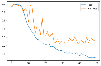
history_frame.loc[:, ['loss', 'val_loss']].plot()
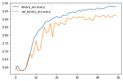
history_frame.loc[:, ['binary_accuracy', 'val_binary_accuracy']].plot();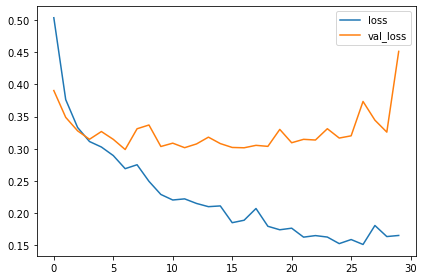 |
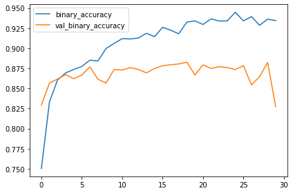 |
첫 수업에 있던 모델의 training과 validation 곡선(learning curves)은 가파르게 갈라졌습니다. 이는 과적합이니 몇 가지 정규화를 적용해야합니다. 이 모델의 learning curve는 이제는 갈라지지 않고 함께 붙어있을 수 있습니다.
특히 validation loss와 accuracy에서 많이 향상된 것으로 보아 augmentation을 적용하면 나아진 것을 확인할 수 있습니다.
Exercise
무작위로 변형을 하면 결과가 어떻게 되는지 보겠습니다.
주어진 데이터에 적절한 augmentation이 무엇일지 고민해보세요.
# Setup feedback system
from learntools.core import binder
binder.bind(globals())
from learntools.computer_vision.ex6 import *
from tensorflow import keras
from tensorflow.keras import layers
from tensorflow.keras.layers.experimental import preprocessing
# Imports
import os, warnings
import matplotlib.pyplot as plt
from matplotlib import gridspec
import numpy as np
import tensorflow as tf
from tensorflow.keras.preprocessing import image_dataset_from_directory
# Reproducability
def set_seed(seed=31415):
np.random.seed(seed)
tf.random.set_seed(seed)
os.environ['PYTHONHASHSEED'] = str(seed)
os.environ['TF_DETERMINISTIC_OPS'] = '1'
set_seed()
# Set Matplotlib defaults
plt.rc('figure', autolayout=True)
plt.rc('axes', labelweight='bold', labelsize='large',
titleweight='bold', titlesize=18, titlepad=10)
plt.rc('image', cmap='magma')
warnings.filterwarnings("ignore") # to clean up output cells
# Load training and validation sets
ds_train_ = image_dataset_from_directory(
'../input/car-or-truck/train',
labels='inferred',
label_mode='binary',
image_size=[128, 128],
interpolation='nearest',
batch_size=64,
shuffle=True,
)
ds_valid_ = image_dataset_from_directory(
'../input/car-or-truck/valid',
labels='inferred',
label_mode='binary',
image_size=[128, 128],
interpolation='nearest',
batch_size=64,
shuffle=False,
)
# Data Pipeline
def convert_to_float(image, label):
image = tf.image.convert_image_dtype(image, dtype=tf.float32)
return image, label
AUTOTUNE = tf.data.experimental.AUTOTUNE
ds_train = (
ds_train_
.map(convert_to_float)
.cache()
.prefetch(buffer_size=AUTOTUNE)
)
ds_valid = (
ds_valid_
.map(convert_to_float)
.cache()
.prefetch(buffer_size=AUTOTUNE)
)
Found 5117 files belonging to 2 classes.
Found 5051 files belonging to 2 classes.
(Optional) Explore Augmentation
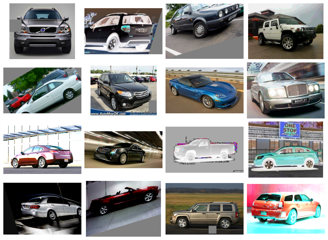
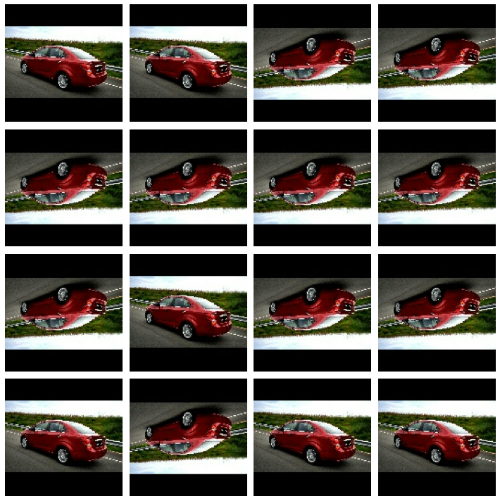
원하는 변형 방식을 선택하고 매개변수도 바꿔보며 코드를 실행하여 얻은 랜덤 이미지를 관찰하세요.
(factor 매개변수는 변한 비율을 나타내며 무조건 0보다 크고 1보다 작습니다.)
선택한 변형 방식이 Car or Truck 데이터셋에 합리적인 보세요.
# all of the "factor" parameters indicate a percent-change
augment = keras.Sequential([
# preprocessing.RandomContrast(factor=0.5),
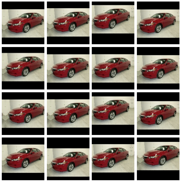
preprocessing.RandomFlip(mode='horizontal'), # meaning, left-to-right
# preprocessing.RandomFlip(mode='vertical'), # meaning, top-to-bottom
# preprocessing.RandomWidth(factor=0.15), # horizontal stretch
# preprocessing.RandomRotation(factor=0.20),
# preprocessing.RandomTranslation(height_factor=0.1, width_factor=0.1),
])
ex = next(iter(ds_train.unbatch().map(lambda x, y: x).batch(1)))
plt.figure(figsize=(10,10))
for i in range(16):
image = augment(ex, training=True)
plt.subplot(4, 4, i+1)
plt.imshow(tf.squeeze(image))
plt.axis('off')
plt.show()
 randomContrast |
 |
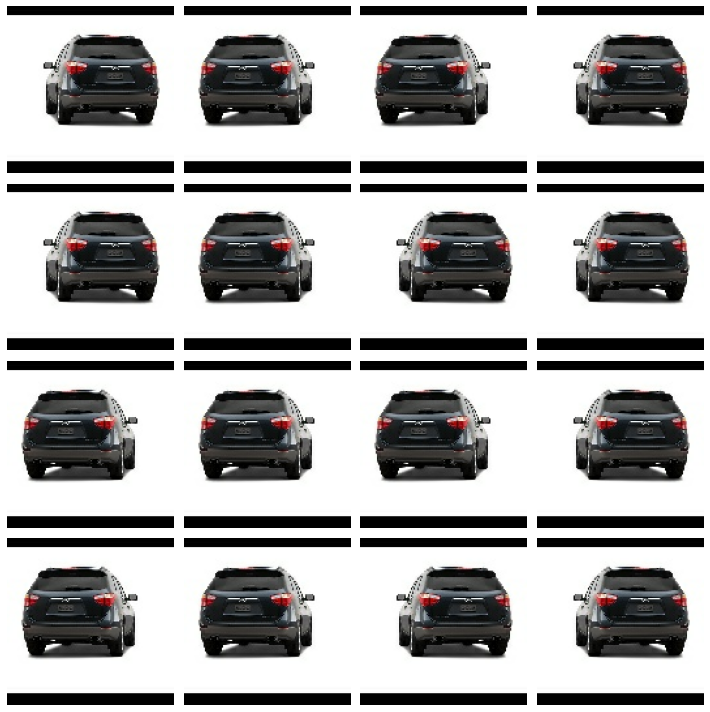 RandomFlip - horizontal == left to right |
 |
 |
 |
Think about reasonable augmentation
이번 실습에서는 어떤 종류의 augmentation이 합리적인지 생각해보고 있지요.
아마 당신의 추론은 해결책에서 논의한 내용과 다를 것입니다. 괜찮아요.
이 문제들의 중요한 점은 변형이 어떻게 분류 문제에 상호 작용하는지 생각해보는 것입니다.
더 좋아지는 지 더 나빠지는 지 말이죠.
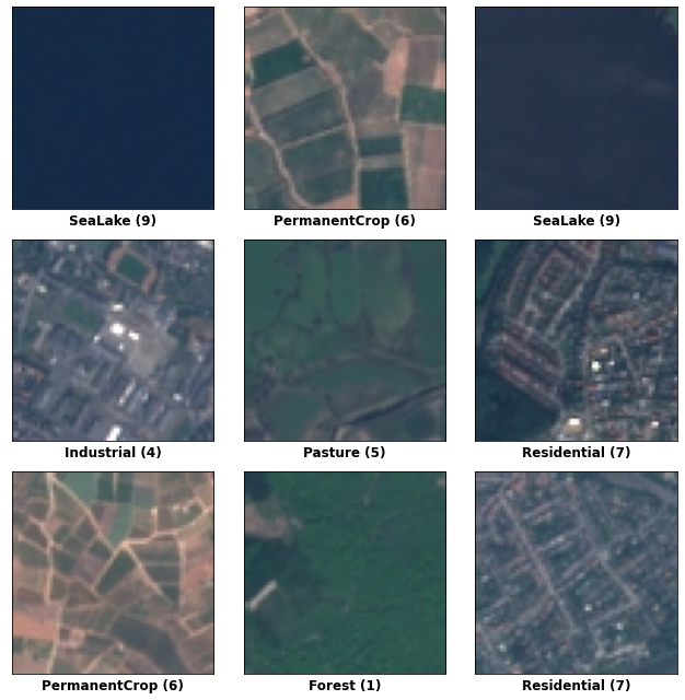
1. EuroSAT
EuroSAT 데이터셋은 지구의 인공위성들의 사진이 담겨 있습니다. 지형지물의 모습에 따라 숫자로 분류되어 있고요.
여기엔 어떤 변형이 적합할까요?
잘 보시면 뒤집히거나 회전되는 변형을 사용하는 것이 좋을 것 같습니다. 왜나면 위에서 아래로 찍었을 때 방위를 잡긴 어려우니깐요. 그
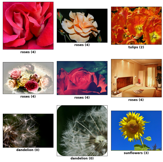
1. TensorFlow Flowers
이 데이터에는 몇 가지 종들의 꽃 사진이 담겨 있습니다.
여기엔 수평 뒤집기나 적당한 회전같은 변형이 좋을 것 같습니다.
꽃의 색깔은 집단마다 구별되기에 색조(hue, like red to blue)의 변화는 아마 성공하기 힘들 것 같네요.
반면에 장미처럼 재배된 꽃은 너무나도 다양하기에 선택한 데이터셋에 따라 이 단점은 개선될 수 있습니다.
Add Preprocessing Layers
이번에는 실습 5에서 만든 costom convnet에 data augmentation을 적용할 것입니다.
data augmentation은 그 크기가 효과적으로 증가하기 때문에 과적합의 위험없이 모델의 용량을 차근차근 증가시킬 수 있습니다.
주어진 모델에 preprocessing layers를 추가해봅시다.
from tensorflow import keras
from tensorflow.keras import layers
model = keras.Sequential([
layers.InputLayer(input_shape=[128, 128, 3]),
# Data Augmentation
preprocessing.RandomContrast(factor=0.10),
preprocessing.RandomFlip(mode='horizontal'),
preprocessing.RandomRotation(factor=0.10),
# Block One
layers.BatchNormalization(renorm=True),
layers.Conv2D(filters=64, kernel_size=3, activation='relu', padding='same'),
layers.MaxPool2D(),
# Block Two
layers.BatchNormalization(renorm=True),
layers.Conv2D(filters=128, kernel_size=3, activation='relu', padding='same'),
layers.MaxPool2D(),
# Block Three
layers.BatchNormalization(renorm=True),
layers.Conv2D(filters=256, kernel_size=3, activation='relu', padding='same'),
layers.Conv2D(filters=256, kernel_size=3, activation='relu', padding='same'),
layers.MaxPool2D(),
# Head
layers.BatchNormalization(renorm=True),
layers.Flatten(),
layers.Dense(8, activation='relu'),
layers.Dense(1, activation='sigmoid'),
])
# Check your answer
q_3.check()
모델을 훈련합시다.
그리고 loss와 accuracy metric을 적용하여 모델을 train set에 맞춰줍시다.
optimizer = tf.keras.optimizers.Adam(epsilon=0.01)
model.compile(
optimizer=optimizer,
loss='binary_crossentropy',
metrics=['binary_accuracy'],
)
history = model.fit(
ds_train,
validation_data=ds_valid,
epochs=50,
)
# Plot learning curves
import pandas as pd

history_frame = pd.DataFrame(history.history)

history_frame.loc[:, ['loss', 'val_loss']].plot()
history_frame.loc[:, ['binary_accuracy', 'val_binary_accuracy']].plot();
 |
 |
training curves를 관찰해보세요. 과적합인가요?
모델의 성능을 이전 수업 때 훈련한 모델과 비교해보면 향상되었나요?
이번 모델에서 learning curves는 꽤나 함께 붙어 있습니다. 이는 augmentation이 과적합을 막아주고 모델을 향샹시키기도 한다는 점을 증명해주네요.
이번 모델의 accuracy는 지금까지 만든 모델 중 가장 높습니다!
항상 그렇지는 않지만 잘 설계한 custom convnet은 이미 훈련된 모델보다 훨씬 나을 때도 있습니다.
'Machine Learning > [Kaggle Course] ML (+ 딥러닝, 컴퓨터비전)' 카테고리의 다른 글
| [생활코딩/CNN] Conv2D (0) | 2021.07.28 |
|---|---|
| [생활코딩/CNN] Flatten (0) | 2021.07.20 |
| Custom Convnets (Convolutional Blocks) (0) | 2021.04.10 |
| The Sliding Window (0) | 2021.04.10 |
| Maximum Pooling - feature extraction (0) | 2021.04.09 |