이전 시간에 convolutional classifier에는 convolutional base와 dense layer로 구성된 head가 있다고 배웠습니다.
base는 이미지에서 시각적 특징을 추출하며 head는 이를 이용해 이미지를 분류합니다.
이번에는 base에 사용되는 두 종류의 layer를 배워보려 합니다.
하나는 ReLU activation을 적용한 convolutional layer이고, 다른 하나는 maximum pooling layer 입니다.
5번째 수업에서 특징 추출을 수행하는 단계에 사용되는 이러한 레이어들로 구성된 자신만의 convnet을 설계하는 법에 대해서 배울 예정입니다.
이번 시간은 ReLU activation을 적용한 convolutional layer만 보겠습니다.
Feature Extraction
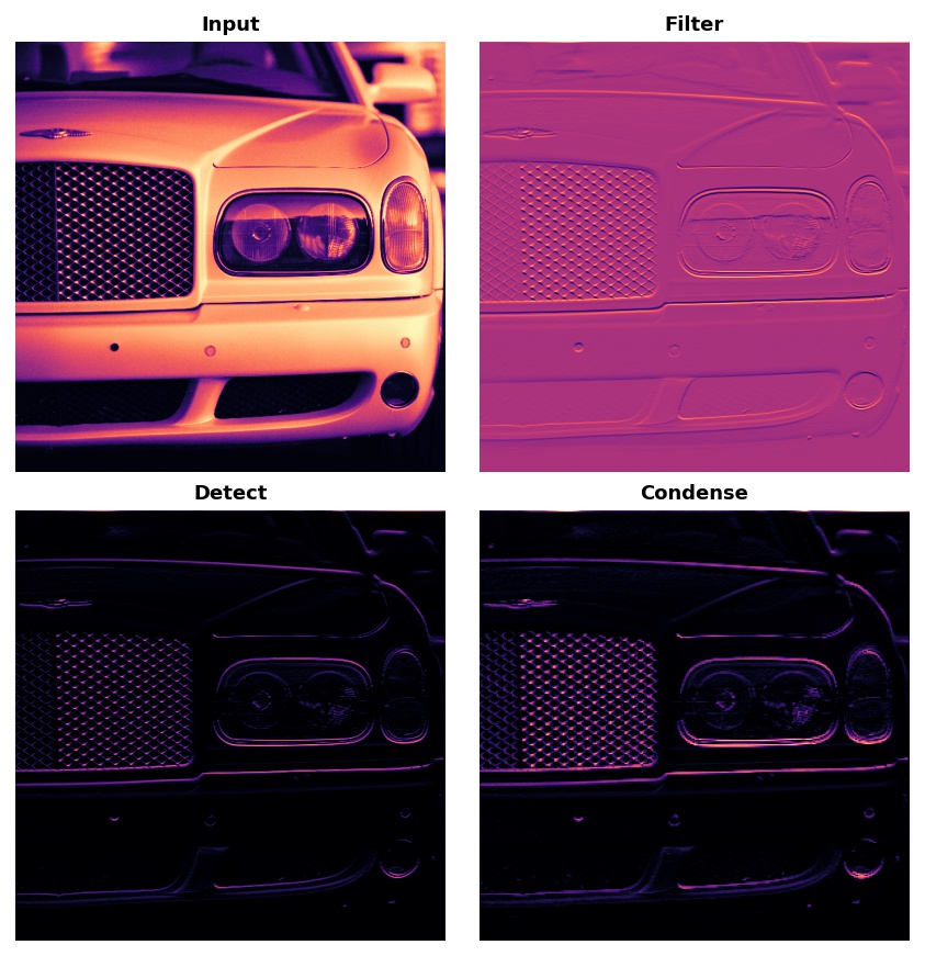
먼저 convolution, ReLU, maximum pooling이 특징 추출 과정에 어떻게 사용되는지 봅시다.
- Convolution : Filter 어떤 특징을 이미지로부터 걸러낸다
- ReLU : Detect 걸러낸 이미지 속에서 특징을 감지
- Maximum Pooling : Condense 특징을 부각시키기 위해 이미지를 압축
보통 네트워크는 하나의 이미지에서 여러 방식의 추출을 동시에, 병렬적으로 수행합니다. 현대의 convnets에서 base의 마지막 레이어가 1000개 이상의 서로 구별되는 시각적 특징들을 생성하는 것은 드문 일이 아닙니다.
Filter with Convolution
filtering 단계를 위해 Kerase에서 convolutional layer를 정의하는 방법은 다음과 같습니다.
아래에 사용된 입력값을 이해하려면 가중치(weight)와 활성화(activation) 레이어의 관계에 대해서 알아야 합니다.
from tensorflow import keras
from tensorflow.keras import layers

model = keras.Sequential([
    layers.Conv2D(filters=64, kernel_size=3), # activation is None
    # More layers follow
])

Kernel == covnets' weight
convnet의 가중치는 훈련이 진행되는 동안 학습을 합니다. 가중치는 해당 convolutional layer에서 포함되어 있습니다.
이러한 weight를 Kernels라 부릅니다. 이는 작은 배열로 표현할 수 있습니다.

Kernel은 이미지를 스캔하여 픽셀 값들의 가중치합을 구합니다.
이런 식으로 Kernel은 일종의 편광 렌즈처럼 작동하여, 특정 정보의 패턴을 강조하거나 약하게 합니다.
Kernel은 convolutional layer가 다음 layer와 연결되는 방식을 정의합니다.
오른쪽 그림 속 kernel은 출력에 있는 하나의 신경(뉴런)을 입력에 있는 9개의 신경(뉴런)에 연결합니다.
kernel_size로 커널의 차원을 설정하여 이러한 연결 방식을 정합니다.
대부분의 kernel은 홀수 개의 차원을 가집니다 (3,3) or (5,5)
그렇기에 중앙에는 하나의 픽셀이 위치할 수 있습니다.
또한, convolutional layer 속 kernel은 생성된 특징들의 종류를 결정합니다.
훈련이 진행되는 동안, convnet은 분류에 필요한 특징은 무엇인지 학습하려 합니다.
이는 그 convnet의 kernel에 최적화된 값을 찾는다는 의미입니다.
Activations
network 속 activation은 feature map으로 부릅니다. filter를 하나의 이미지에 적용했을 때의 결과입니다.
커널이 추출한 시각적 특징을 담고 있습니다.

커널 속 패턴의 숫자를 보며 생성된 feature map을 구별할 수 있습니다.
보통 convolution이 입력값에 있는 강조된 무언가는 커널 속 양수의 분포와 매치됩니다.
왼쪽과 오른쪽 커널은 모두 수평 모양을 추출해냈습니다.
Detect with ReLU(=rectified)

filterling 후에는, feature maps가 activation function을 통과합니다.
rectifier function은 다음과 같은 그래프를 가지게 됩니다.
음수 영역에 0이기에 rectified라는 명칭이 붙었습니다.
rectifier가 적용된 뉴런은 rectified linear unit으로 부릅니다.
rectifier function은 ReLU activation 또는 ReLU function으로 부릅니다.
ReLU activation은 Activation layer에서 정의되지만 대부분 Conv2D의 activation function에 포함되어 있습니다.
model = keras.Sequential([
    layers.Conv2D(filters=64, kernel_size=3, activation='relu')
    # More layers follow
])
활성화 함수를 중요도에 따라 매겨진 픽셀값들을 등급/순서를 매기는 용도로 생각할 수도 있습니다.
ReLU 활성화 함수에서 음수는 중요하지 않음을 의미하기에 0으로 지정합니다.
아래 사진은 feature maps에 적용된 ReLU입니다.
특정 특징(feature)을 고립시키고 분리해낸 걸 어떻게 성공했는지 관찰해보세요.
다른 활성화 함수와 마찬가지로 ReLU 함수도 nonlinear, 비선형 방식입니다.
이는 네트워크 속 모든 레이어의 최종 결과는 이 결과에 무엇을 추가하였는지에 따라 점점 달라질 것입니다.
이는 하나의 레이어에서도 해냈던 것과 비슷할 것입니다.
비선형성은 특징들이 네트워크 속에서 좀 더 깊게 깊게 흥미로운 방식으로 결합한다는 사실을 증명합니다.
(Feature compounding 참고)

Example - Convolution과 ReLU 적용하기

이번 예제는 convolutional networks가 어떻게 작동되는지 그 숨겨진 과정을 이해하기 위한 예제입니다.
아래는 사용될 이미지를 가져오는 코드입니다.
import tensorflow as tf
import matplotlib.pyplot as plt
plt.rc('figure', autolayout=True)
plt.rc('axes', labelweight='bold', labelsize='large',
       titleweight='bold', titlesize=18, titlepad=10)
plt.rc('image', cmap='magma')

image_path = '../input/computer-vision-resources/car_feature.jpg'
image = tf.io.read_file(image_path)
image = tf.io.decode_jpeg(image)

plt.figure(figsize=(6, 6))
plt.imshow(tf.squeeze(image), cmap='gray')
plt.axis('off')
plt.show();
필터링 단계를 위해 커널을 정의하고 거기에 convolution을 적용해야 합니다.
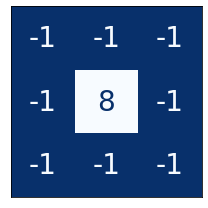
이번 예제에 사용되는 커널은 'edge detection" 커널입니다.
tf.constant로 정의할 수 있으며, np.array처럼 정의됩니다.
이는 TensorFLow에서 사용되는 하나의 tensor를 생성합니다.
import tensorflow as tf

kernel = tf.constant([
    [-1, -1, -1],
    [-1,  8, -1],
    [-1, -1, -1],
])

plt.figure(figsize=(3, 3))
show_kernel(kernel)
텐서플로우는 tf.nn 모듈 속에 신경망에 사용되는 수많은 연산을 가지고 있습니다.
우리는 conv2d와 relu를 써볼 것입니다.
이들은 Keras 레이어의 간단한 함수 버전입니다.
아래 코드는 텐서플로우에 적합한 코드로 변환(reformatting)하는 내용입니다.
# Reformat for batch compatibility.
image = tf.image.convert_image_dtype(image, dtype=tf.float32)
image = tf.expand_dims(image, axis=0)
kernel = tf.reshape(kernel, [*kernel.shape, 1, 1])
kernel = tf.cast(kernel, dtype=tf.float32)
커널을 적용하고 그 결과를 보여주는 코드입니다.

image_filter = tf.nn.conv2d(
    input=image,
    filters=kernel,
    # we'll talk about these two in lesson 4!
    strides=1,
    padding='SAME',
)

plt.figure(figsize=(6, 6))
plt.imshow(tf.squeeze(image_filter))
plt.axis('off')
plt.show();
다음은 ReLU 함수를 이용한 감지(detection) 단계입니다.
매개변수를 필요로 하지 않기에 convolution보다 간단한 함수입니다.

image_detect = tf.nn.relu(image_filter)

plt.figure(figsize=(6, 6))
plt.imshow(tf.squeeze(image_detect))
plt.axis('off')
plt.show();
이번 시간에는 feature map을 생성해봤습니다.
자동차의 특징이나 트럭의 특징을 잘 살리는 feature를 생성한 것입니다.
훈련하는 동안 convnet은 이러한 features를 찾아내는 kernel을 생성했습니다.
convnet에서는 두 단계로 특징을 추출하는 일을 수행합니다.
Conv2D 레이어로 filtering을 하고 relu activation으로 감지합니다.
Exercise
이 예제를 통해 feature extraction에 필요한 직감을 가져보려 합니다.
그러니 커널은 당신이 선택해보세요.
이번 코스는 이미지를 다루는 내용이지만, 연산 과정을 이해하려면 수학을 배워야 합니다.
그래서 어떻게 feature maps가 숫자로 구성된 배열을 나타내는지, 그리고 커널과 함께 convolution을 쓰면 그 결과가 어떠한지도 봅시다.
# Setup feedback system
from learntools.core import binder
binder.bind(globals())
from learntools.computer_vision.ex2 import *

import numpy as np
import tensorflow as tf
import matplotlib.pyplot as plt

plt.rc('figure', autolayout=True)
plt.rc('axes', labelweight='bold', labelsize='large',
       titleweight='bold', titlesize=18, titlepad=10)
plt.rc('image', cmap='magma')

tf.config.run_functions_eagerly(True)
Apply Transformations
이번 수업에 쓰일 사진을 불러오는 내용입니다.

image_path = '../input/computer-vision-resources/car_illus.jpg'
image = tf.io.read_file(image_path)
image = tf.io.decode_jpeg(image, channels=1)
image = tf.image.resize(image, size=[400, 400])

img = tf.squeeze(image).numpy()
plt.figure(figsize=(6, 6))
plt.imshow(img, cmap='gray')
plt.axis('off')
plt.show();
이미지 처리 과정에 사용되는 기본적인 커널들은 다음과 같습니다.
import learntools.computer_vision.visiontools as visiontools
from learntools.computer_vision.visiontools import edge, bottom_sobel, emboss, sharpen

kernels = [edge, bottom_sobel, emboss, sharpen]
names = ["Edge Detect", "Bottom Sobel", "Emboss", "Sharpen"]

plt.figure(figsize=(12, 12))
for i, (kernel, name) in enumerate(zip(kernels, names)):
    plt.subplot(1, 4, i+1)
    visiontools.show_kernel(kernel)
    plt.title(name)
plt.tight_layout()
1. Define Kernel
커널 속 숫자의 총합은 결과 이미지의 밝기를 결정한다는 점을 기억하세요.
일반적으로 숫자의 총합은 0~1 사이를 유지하도록 해야합니다. (정답을 위해 필수적인 절차는 아닙니다)
하나의 커널은 수많은 행과 열을 가질 수 있습니다. 이번 예제에서는 3x3 커널을 이용하려 합니다.
tf.constant를 적용한 커널을 정의해보세요.
(Emboss 커널을 선택해봤어요)
kernel = tf.constant([ ##Emboss
    [-2, -1, 0],
    [-1,1,1],
    [0,1,2],
])
# Uncomment to view kernel
# visiontools.show_kernel(kernel)
# Reformat for batch compatibility and tensorflow.
image = tf.image.convert_image_dtype(image, dtype=tf.float32)
image = tf.expand_dims(image, axis=0)
kernel = tf.reshape(kernel, [*kernel.shape, 1, 1])
kernel = tf.cast(kernel, dtype=tf.float32)
2. Feature Extraction
2-1. Apply Convolution 2D layer
#Give the TensorFlow convolution function (without arguments)
conv_fn = tf.nn.conv2d
image_filter = conv_fn(
input=image,
filters=kernel,
strides=1, # or (1, 1)
padding='SAME',
)
plt.imshow(
# Reformat for plotting
tf.squeeze(image_filter)
)
plt.axis('off')
plt.show();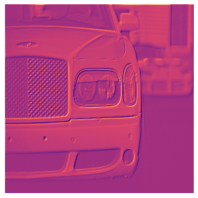 |
 |
 |
 |
2-2. Apply ReLU activation function
# YOUR CODE HERE: Give the TensorFlow ReLU function (without arguments)
relu_fn = tf.nn.relu
image_detect = relu_fn(image_filter)

plt.imshow(
    # Reformat for plotting
    tf.squeeze(image_detect)
)
plt.axis('off')
plt.show();
옆의 사진은 당신이 선택한 커널이 생성해준 feature map입니다.
마음에 든다면, 위의 다른 커널들도 적용해보고,
특정 feature를 추출하는 것도 만들어보세요
 |
 |
 |
 |
3. Observe Convolution on a Numerical Matrix
커널과 feature maps의 결과는 시각적으로 확인할 수 있습니다. Conv2D와 ReLU의 결과를 통해서 말이죠.
그런데 convolutional network( 그냥 모든 신경망) 속 연산은 수학적인 함수로 되어있습니다.
이제부터는 이 숫자들을 읽는 관점에 대해 배워보려 합니다.
하나의 이미지를 나타내는 간단한 배열 하나와 커널을 나타내는 또다른 배열, 총 두 개를 정의합시다.
# Sympy is a python library for symbolic mathematics. It has a nice
# pretty printer for matrices, which is all we'll use it for.
import sympy
sympy.init_printing()
from IPython.display import display

image = np.array([
    [0, 1, 0, 0, 0, 0],
    [0, 1, 0, 0, 0, 0],
    [0, 1, 0, 0, 0, 0],
    [0, 1, 0, 0, 0, 0],
    [0, 1, 0, 1, 1, 1],
    [0, 1, 0, 0, 0, 0],
])

kernel = np.array([
    [1, -1],
    [1, -1],
])

display(sympy.Matrix(image))
display(sympy.Matrix(kernel))
# Reformat for Tensorflow
image = tf.cast(image, dtype=tf.float32)
image = tf.reshape(image, [1, *image.shape, 1])
kernel = tf.reshape(kernel, [*kernel.shape, 1, 1])
kernel = tf.cast(kernel, dtype=tf.float32)
 두번째열, 그리고 5번째 행에 줄이 생기게 됨 |
 이 커널을 이미지에 적용하면 어떤 결과가 나타날까? |
 |
 |
커널을 해석하는 방법은 1의 위치에 따른 모양을 읽는 것입니다.
그 1이 나타내는 그림을 하나의 feature로 봅니다.
필터를 조정하면
image_filter = tf.nn.conv2d(
    input=image,
    filters=kernel,
    strides=1,
    padding='VALID',
)
image_detect = tf.nn.relu(image_filter)

# The first matrix is the image after convolution, and the second is
# the image after ReLU.
display(sympy.Matrix(tf.squeeze(image_filter).numpy()))
display(sympy.Matrix(tf.squeeze(image_detect).numpy())) |
 |


'Machine Learning > [Kaggle Course] ML (+ 딥러닝, 컴퓨터비전)' 카테고리의 다른 글
| The Sliding Window (0) | 2021.04.10 |
|---|---|
| Maximum Pooling - feature extraction (0) | 2021.04.09 |
| Convolutional Classifier (0) | 2021.03.29 |
| [Kaggle Course] Binary Classification(이진 분류) - sigmoid, cross-entropy (0) | 2020.12.30 |
| [Kaggle Course] Dropout, Batch Normalization (0) | 2020.12.26 |